A Case Study on the Relationship between Police Residence and Fatal Police Shootings
Gabriel Brock | Fa23 | Harvard University
On average, police in the United States shoot and kill more than 1,000 people every year…and then they go home to their families
Abstract
This case study investigates the intricate relationship between police residence and fatal police shootings, employing a data science approach to uncover insights and patterns within the context of law enforcement agencies. Focused on police officers residing in the cities they serve, the study examines whether this residency factor correlates with the incidence of fatal police shootings. The data set, spanning the years 2015 to 2023, is composed of information on police agencies involved in at least one fatal shooting, and is subjected to rigorous analysis using advanced statistical methods and machine learning techniques.
This study aims to discern patterns, trends, and potential biases associated with the geographical proximity of police officers to the communities they police. A comprehensive exploration of demographic, socioeconomic, and policing variables contributes to a nuanced understanding of the factors influencing fatal police shootings. Furthermore, the study seeks to identify any disparities in incident rates based on officers’ residency status, considering variables such as race, community demographics, and departmental policies.
The insights derived from this case study bear substantial implications for informing public policy, refining police training protocols, and strengthening community relations. By unraveling the nuanced dynamics surrounding police residence and fatal police shootings, this case study aims to provide evidence-based recommendations to enhance transparency, accountability, and trust between law enforcement agencies and the communities they serve. In doing so, it contributes to the broader discourse on police reform, fostering a data-driven approach to address critical issues and promote safer, more resilient communities.
Hypotheses
We will conduct two hypothesis tests to analyze both;
The nominal relationship between an increasing proportion of in-city officer residency and number of fatal police shooting deaths
\(H_0\): The mean total number of fatal shootings per agencies does not differ based on if a majority of the officers live in the city or not.
\(H_A\): The mean total number of fatal shootings per agencies is fewer in cities where a majority of the officers live in the city then cities where they do not.
The categorical difference in fatal police shooting deaths between cities where a majority or or minority of police officers live in the city.
\(H_0\): There is no relationship between percentage of the total police force that lives in the city they serve and number of fatal shootings.
\(H_A\): There is a relationship between percentage of the total police force that lives in the city they serve and number of fatal shootings.
\(H_0 : \rho = 0\)
\(H_0 : \rho \neq 0\)
Methods
Tidying Data
Show the code
##Tidying Data#creating dfs from .csv filespolice_locals <-read_csv("data/police-locals.csv")agencies <-read_csv("data/fatal-police-shootings-agencies.csv")shootings <-read_csv("data/fatal-police-shootings-data.csv")#removing old `city` tag from data set that we created when decatenated the city namespolice_locals <- police_locals |>select(-city_old)# creating `agencies` df with just police departmentsagencies <- agencies |>filter(grepl("department", tolower(name))) |>filter(!grepl("county", tolower(name)))#creating binned categorical account of if shooting victim was `armed`shootings <- shootings |>mutate(armed =case_when(is.na(armed_with) ~"NO", armed_with =="unarmed"~"NO", armed_with =="unknown"~"NO", armed_with =="undetermined"~"NO", armed_with =="gun"~"YES", armed_with =="knife"~"YES", armed_with =="blunt_object"~"YES", armed_with =="other"~"YES", armed_with =="replica"~"YES", armed_with =="vehicle"~"YES"))#creating df with only agency `names`, `id`, and `state`agencies_ids <- agencies |>select(name, id, state)#creating df with `city`, `agency`, and `state` info for each shootingshooting_agencies <- shootings |>select(city, agency_ids, state)#changing `shooting` var in `shooting_agencies` df to numericshooting_agencies$agency_ids <-as.numeric(shootings$agency_ids)#creating df with `city` and `state` info for each agency by joining `agencies_ids` and `shooting_agencies`agencies_w_cities <- agencies_ids |>left_join(shooting_agencies, by =c("id"="agency_ids", "state"="state")) |>drop_na(city) |>distinct(id, .keep_all =TRUE)#creating df with census data for each agency by joining `agencies_w_cities` and `police_locals`agencies_census <- agencies_w_cities |>full_join(police_locals, by =c("city"="city", "state"="state")) |>drop_na(police_force_size) |>distinct(id, .keep_all =TRUE) |>mutate(majority =if_else(all >=0.5, "TRUE", "FALSE"))#creating df of only shootings involving agencies within `agencies` dfshootings_case <- shootings |>right_join(agencies_census, by =c("city"="city", "state"="state")) |>select(-agency_ids) |>rename(agency_ids = id.y, id = id.x, agency = name.y, victim = name.x) |>select(-location_precision, -race_source)
Counting Shootings
Show the code
#count shootings by agencyshootings_by_agency <- shootings_case |>count(agency)#find top 25 agencies with the most shootingstop_25_agencies <- shootings_by_agency |>slice_max(n, n =25)
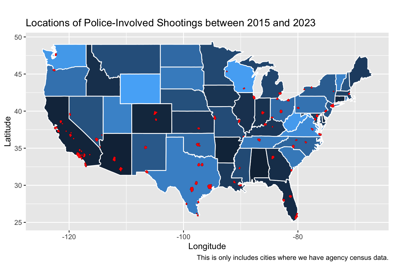
Mapping Locations of Police-Involved Shootings between 2015 and 2023
Show the code
shot_map
Show the code
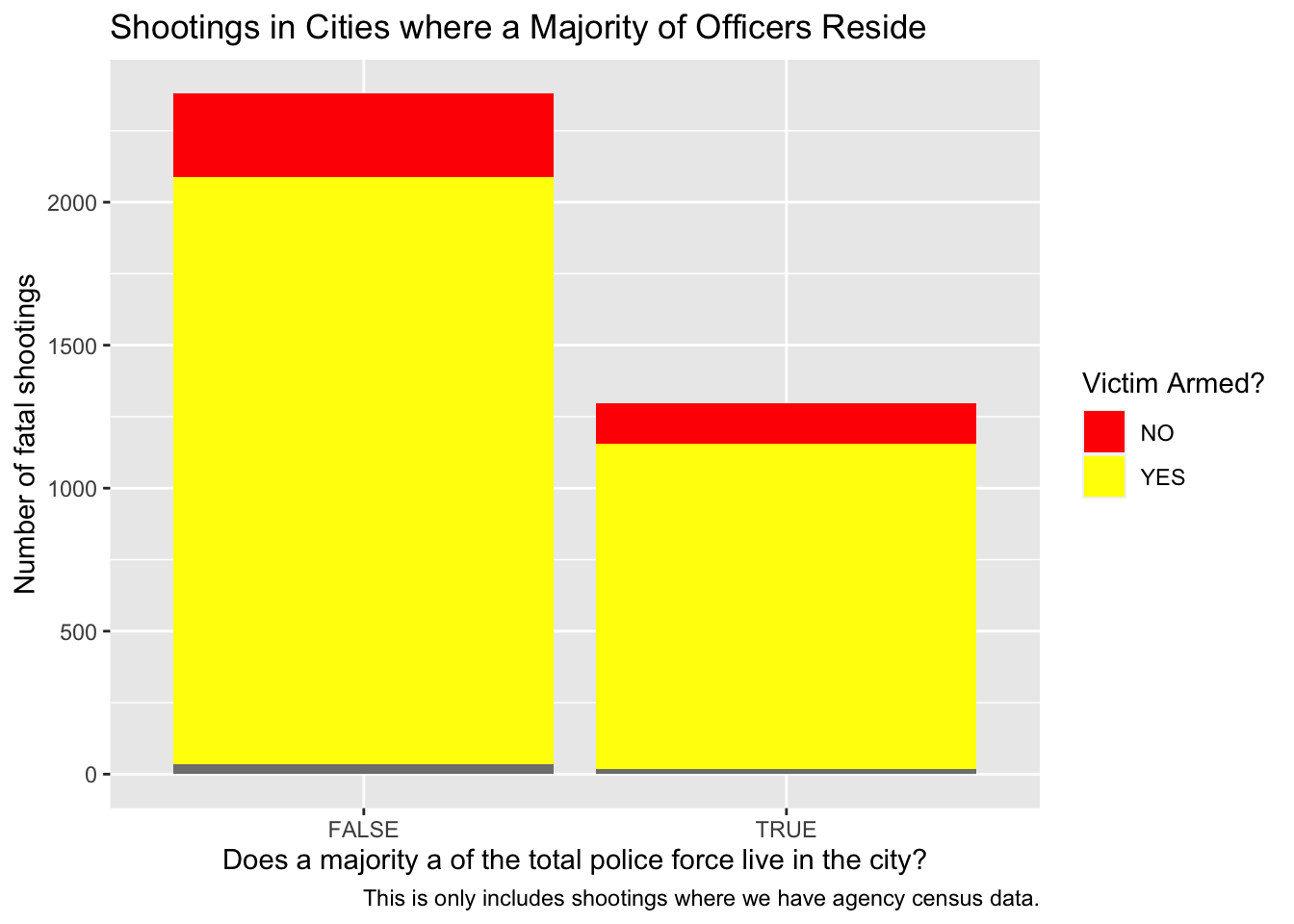
#creating df with total shootings per agency and census dataagencies_census <- agencies_census |>left_join(shootings_by_agency, by =c("name"="agency"))#creating visualization of comparison Shootings in Cities where a Majority/Minority of Officers Residep0 <- shootings_case |>ggplot(aes(x = majority, fill = armed)) +geom_bar() +labs(title ="Shootings in Cities where a Majority of Officers Reside",caption ="This is only includes shootings where we have agency census data.",x ="Does a majority a of the total police force live in the city?",y ="Number of fatal shootings",fill ="Victim Armed?") +scale_fill_manual(values =c(NO ="Red",YES ="Yellow"))
Show the code
p0
Show the code
#calculate mean number of shootings per agency in cities where a majority of officers reside in the citymajority_mean <- shootings_case |>filter(majority ==TRUE) |>count(agency) |>summarize(maj_mean =mean(n))#calculate mean number of shootings per agency in cities where a minority of officers reside in the cityminority_mean <- shootings_case |>filter(majority ==FALSE) |>count(agency) |>summarize(min_mean =mean(n))#calculate a difference in means between the `majority` and `minority`diff_in_means <- majority_mean - minority_mean
Show the code
#tidy tableknitr::kable(head(diff_in_means))
maj_mean
-2.575
Show the code
#fit single linear regression model for correlation between percentage of officer residency and number of fatal shootings per agencyfit <-lm(n ~ all, data = agencies_census)#add `armed` and `majority` to `shootings_by_agency` dfshootings_by_agency_census <- shootings_case |>group_by(agency) |>count(armed) |>drop_na(n, armed) |>right_join(agencies_census, by =c("agency"="name")) |>distinct(armed, .keep_all =TRUE)shootings_by_agency_census <- shootings_by_agency_census |>select(n.x, armed, all) #fit multiple linear regression model for correlation between percentage of officer residency and victim armament and number of fatal shootings per agencyfit_multi <-lm(n.x ~ all + armed, data = shootings_by_agency_census)
Results
Multiple Linear Regression of relationship between percentage of officer residency and number of fatal shootings per agency fit
The model equation for fit is:
\[
\text{Number of Fatal Shootings (n)} = 35.7782 - 0.5874 \times \text{Percentage of Officer Residency (all)}
\]
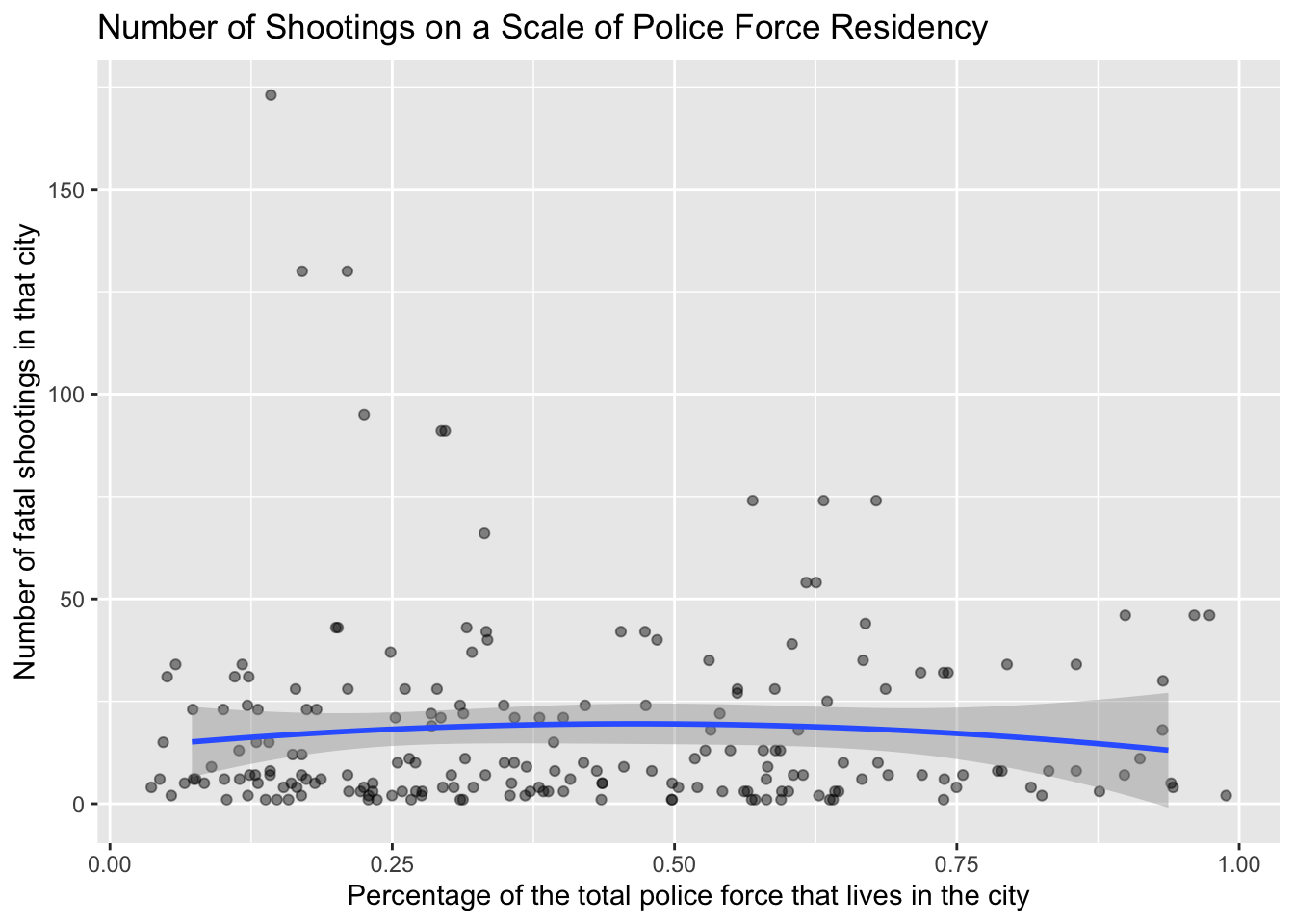
The intercept, \(35.7782\), is the estimated number of fatal shootings when the percentage of officer in-city residency (all) is \(0\). For each one-unit increase in the percentage of officer residency, the number of fatal shootings is expected to decrease by \(0.5874\) (\(-0.5874\)) units, assuming all other factors remain constant.
This model suggests that there is a negative association between the percentage of officer residency and the number of fatal shootings. However, it’s important to interpret the results in the context of your data and consider potential confounding factors, like whether or not the victim was armed.
Show the code
#visualize polynomial relationship between percentage of officer residency and number of fatal shootings per agencyggplot(data = shootings_by_agency_census, aes(x = all, y = n.x)) +geom_jitter(width =0.10, height =0, alpha =0.45) +geom_smooth(method ="lm", formula = y ~poly(x, 2), se =TRUE) +labs(title ="Number of Shootings on a Scale of Police Force Residency",x ="Percentage of the total police force that lives in the city",y ="Number of fatal shootings in that city")
Multiple Linear Regression of relationship between percentage of officer residency/victim armament and number of fatal shootings per agency fit_multi
The model equation for fit_multi considering victim armament (armed) is:
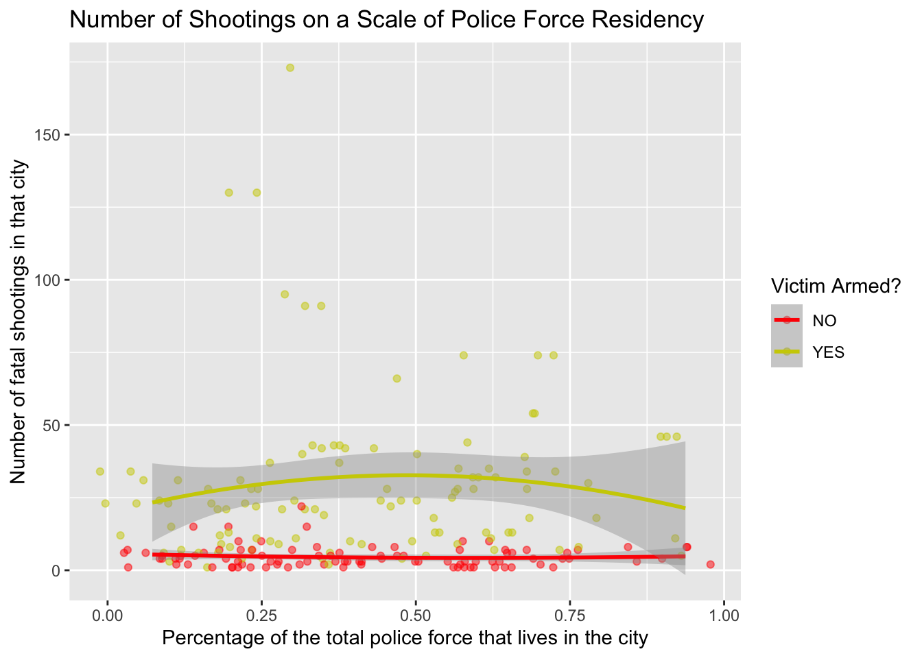
The intercept, \(4.117\), is the estimated number of fatal shootings where the percentage of officer in-city residency (all) is \(0\) and the victim was un-armed. For each one-unit increase in the percentage of in-city officer residency compared to the total force (all), we expect an increase of\(1.211\) fatal shootings, assuming the victim’s armament status (armed:YES) remains constant.
The coefficient for ‘armedYES’, \(24.921\), indicates that the victim is armed (armed:YES), we expect an increase of\(24.921\) fatal shootings compared to when the victim is not armed (armed is No), assuming the percentage of officer residency (all) remains constant.
In summary, the model suggests that the percentage of officer residency and whether the victim is armed are associated with the number of fatal shootings per agency even as we control for victim armament. However, as correlation does not imply causation, and other factors not included in the model may influence the outcomes.
Show the code
#visualize polynomial relationship between percentage of officer residency and victim armament and number of fatal shootings per agencyggplot(data = shootings_by_agency_census, aes(x = all, y = n.x, color = armed)) +geom_jitter(width =0.10, height =0, alpha =0.5) +geom_smooth(method ="lm", formula = y ~poly(x, 2), se =TRUE) +labs(title ="Number of Shootings on a Scale of Police Force Residency",x ="Percentage of the total police force that lives in the city",y ="Number of fatal shootings in that city",color ="Victim Armed?") +scale_color_manual(values =c(NO ="Red",YES ="Yellow3"))
Show the code
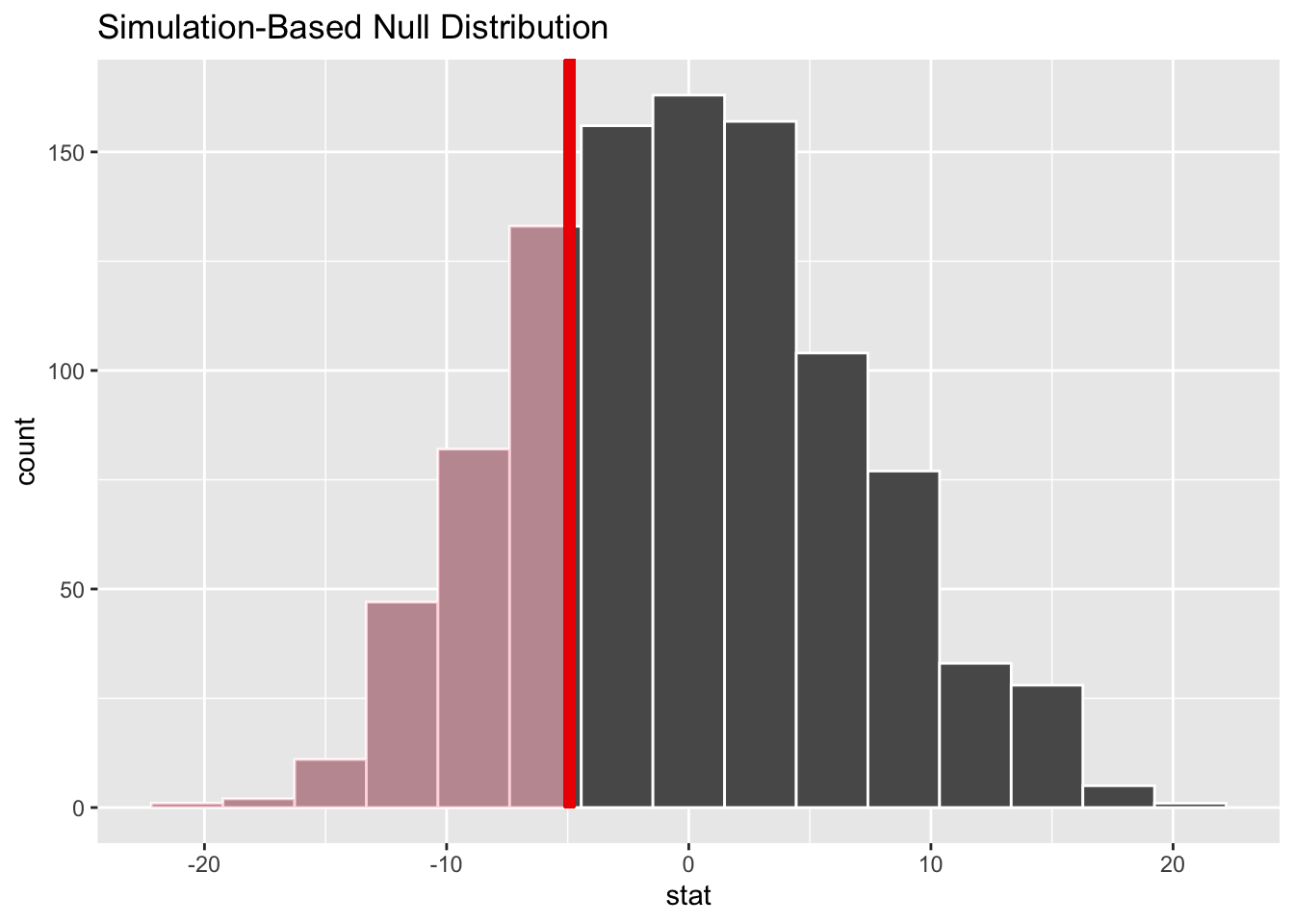
#generate null distributionnull_dist <- agencies_census |>specify(n ~ majority) |>hypothesize(null ="independence") |>generate(reps =1000, type ="permute") |>calculate(stat ="diff in means", order =c("TRUE", "FALSE"))#compute observed test statistictest_stat <- agencies_census |>specify(n ~ majority) |>calculate(stat ="diff in means", order =c("TRUE", "FALSE"))#visualize p-valuenull_dist |>visualize() +shade_p_value(obs_stat = test_stat, direction ="less")
Show the code
#compute p-value p_diff <- null_dist |>get_p_value(obs_stat = test_stat, direction ="less")
Show the code
#tidy tableknitr::kable(head(p_diff))
p_value
0.256
At a significance level of \(\alpha = 0.05\), the p-value of \(0.248\) suggests that, there is insufficient evidence to reject the null hypothesis. In this context, since our null hypothesis asserts that mean total number of fatal shootings per agencies does not differ based on if a majority of the officers live in the city or not, our p-value indicates that, assuming our null is true, the probability of observing our given test statistic (difference in means; \(\mu_{maj} − \mu_{min}\)) is \(-4.92\) is around \(25\%\) (\(0.248\)). Meaning our observed difference in means between the groups is likely to have occurred by random chance.
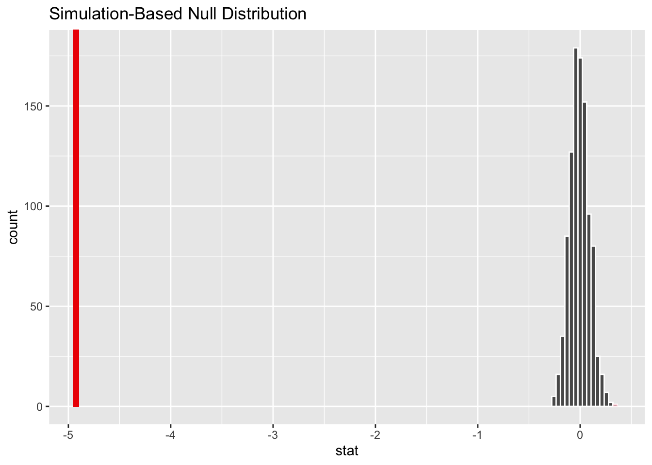
#compute p-valuep_cor <- null_dist_cor |>get_p_value(obs_stat = test_stat, direction ="two.sided")
Show the code
#tidy tableknitr::kable(head(p_cor))
p_value
0
At a significance level of \(\alpha = 0.05\), the p-value of \(0.248\) suggests that, there is sufficient evidence to reject the null hypothesis. In this context, since our null hypothesis asserts that there is no relationship between percentage of the total police force that lives in the city they serve and number of fatal shootings, our p-value indicates that, assuming our null is true, the probability of observing our given test statistic (correlation coefficient; \(\rho = 0\)) is \(-0.0470\) is around \(0\%\) (\(0\)). Meaning our observed correlation coefficient likely would not happen if there was no relationship between percentage of officer residency and number of fatal shootings for a given agency.
Conclusion
General Conclusions
This comprehensive case study delves into the complex interplay between police force in-city residence and fatal police shootings, utilizing a data-driven approach to unearth patterns and insights within the realm of law enforcement agencies. Focused on the residency status of police officers in the cities they serve, the study scrutinizes whether this factor is correlated with the occurrence of fatal police shootings. Covering the years 2015 to 2023 and incorporating information on police agencies involved in at least one fatal shooting, the research employs advanced statistical methods and machine learning techniques to provide a nuanced understanding of the phenomenon.
Key Findings
The analysis reveals a negative association between the percentage of officer residency in a city and the number of fatal shootings, suggesting that, on average, a higher proportion of in-city officer residency is associated with fewer fatal police shootings. However, correlation is not equal to causation so we conducted a multiple linear regression. When controlling for victim armament, the study identifies a complex relationship. While an increase in the percentage of officer residency is associated with fewer fatal shootings, the presence of an armed victim is linked to a significant increase in fatal shootings.
Our hypothesis tests provide insights into the statistical significance of the observed relationships; a difference in mean number of shootings per agency in cities where a majority or minority of officers reside in the city and the nominal relationship (correlation) between an increasing proportion of in-city officer residency and number of fatal police shooting death. The first test suggests that there is insufficient evidence to reject the null hypothesis regarding the difference in mean total fatal shootings between agencies with a majority and minority of officers residing in the city. The second test indicates a significant relationship between the percentage of officer residency and the number of fatal shootings.
Limitations and Considerations and Improvements for Future Study
It’s essential to acknowledge the limitations of this study. The analysis relies on available data, and causation cannot be inferred from correlation. Factors beyond the scope of this study may influence fatal police shootings, emphasizing the need for a holistic approach to police reform.
The accuracy and completeness of the data used in the analysis are dependent on the quality of reporting by law enforcement agencies. Incomplete or inaccurate reporting could introduce biases. The study spans the years 2015 to 2023. Changes in law enforcement practices or societal dynamics over time may not be adequately captured. There may be confounding variables not included in the analysis that could influence the relationship between police residence and fatal police shootings besides residency as we demonstrated in the study.
The study may not account for geographical variations in policing practices. Policing approaches can differ significantly between urban and rural areas, and this variability might affect the observed relationships. The analysis does not control for the population size of the cities being studied. Fatal shootings per agency per capita might provide a more nuanced understanding of the impact on communities. While the study considers the victim’s armament status, the context of each shooting, such as the immediacy of threat and the perceived level of danger, is not fully explored. This nuance could impact the outcomes.
If we had more time, it would be wise to recompile data with information from the 2020 census. It would also be wise to control for city population in future studies, fatal shootings per capita.
Policy Recommendations
The findings of this case study carry substantial implications for policy-making, police training, and community relations. The evidence suggests that fostering a higher percentage of officer residency in the communities they police may contribute to a reduction in fatal police shootings. However, it’s crucial to consider other influential factors, such as victim armament, when formulating comprehensive policies.
Implement measures to enhance transparency and accountability within law enforcement agencies, including the regular monitoring of fatal shooting incidents and the factors influencing them. Encourage community policing strategies that promote stronger bonds between officers and the communities they serve. Initiatives to increase the percentage of officers residing in their assigned cities may contribute to building trust. Prioritize training programs that focus on de-escalation techniques and handling situations involving armed individuals. This can mitigate the escalation of incidents and reduce the likelihood of fatal outcomes. Policy makers and researchers should also promote ongoing research and data collection to monitor trends and assess the effectiveness of implemented strategies. Continued analysis will help refine policies and ensure adaptability to evolving community needs.
In conclusion, this case study contributes to the ongoing discourse on police reform by providing evidence-based insights into the relationship between police residence and fatal police shootings. By addressing these critical issues, we aspire to foster safer, more resilient communities and facilitate positive transformations in law enforcement practices.